Wie wir render-farm-GPUs benchmarken: Eine reproduzierbare Kosten-pro-Frame-Methode (2026)
Überblick
Einleitung
Ein Benchmark-Wert ist leicht zu veröffentlichen und schwer zu vertrauen. Jeder kann „RTX 5090: X Punkte" posten, aber die Zahl, die entscheidet, ob ein Renderjob auf einer Karte oder einer anderen lohnt, ist kein synthetischer Wert — es sind die Kosten pro fertigem Frame. Diese Zahl hängt von der Szene, den Render-Einstellungen, der Render-Engine, dem Treiber und der verwendeten Rechenweise ab, und fast nichts davon ist in einem Leaderboard-Eintrag sichtbar.
Diese Seite ist die Methode, nicht das Leaderboard. Sie dokumentiert, wie wir bei Super Renders Farm render-farm-GPUs benchmarken, damit das Ergebnis aussagekräftig ist: wie wir eine Benchmark-Szene auswählen, welche Render-Einstellungen wir sperren, was wir über die Hardware-Matrix hinweg konstant halten, wie wir rohe Frame-Zeiten in eine belastbare Kosten-pro-Frame-Zahl umwandeln — und den Teil, den die meisten Beiträge überspringen: die expliziten Schritte, damit Dritte die gesamte Methode auf ihrer eigenen Hardware reproduzieren können. Die Ergebnisse dieser Methode haben wir bereits veröffentlicht; dies ist das Rezept dahinter. Wo unten eine Zahl erscheint, handelt es sich um eine reale Zahl aus einer dieser Studien, die als Rechenbeispiel zitiert wird, nicht hier neu hergeleitet.
Synthetische Benchmarks versus produktionsbasierte Kosten pro Frame
Es gibt zwei Ebenen des GPU-Benchmarkings, und ihre Verwechslung ist die Quelle der meisten Verwirrung.
Die erste ist die synthetische Ebene: standardisierte Werkzeuge, die eine feste Szene rendern und eine Punktzahl ausgeben. Cinebench R24, der Chaos V-Ray Benchmark und OctaneBench gehören alle dazu. Sie eignen sich für das relative Ranking — eine einzige wiederholbare Arbeitslast, identisch auf jeder Maschine, sodass Karten nebeneinander aufgestellt werden können. Wie diese Werte zu lesen sind, erläutern wir in unserem V-Ray-Benchmark-Leitfaden und unserem Beitrag zu Cinebench-Werten für Cloud-Rendering. Was ein synthetischer Wert bewusst ausblendet, ist alles, was sich in der Produktion verändert: Ihre Geometrie, Ihr Sampling, Ihr Denoiser, Ihre Ausgabeauflösung und der Pro-Job-Overhead, den eine echte Warteschlange mit sich bringt.
Die zweite ist die Produktionsebene: wie lange ein repräsentativer echter Frame tatsächlich benötigt, und was das kostet. Diese Ebene ist das Ziel dieser Methodik. Ein synthetischer Wert ist ein Eingangsparameter — eine Möglichkeit, eine Ausgangsschätzung zu extrapolieren —, aber er ist nicht die Antwort. Die Brücke zwischen den beiden ist im Prinzip einfach: Eine Maschine, die auf demselben Benchmark-Build etwa doppelt so viele Punkte wie eine andere erreicht, rendert einen vergleichbaren Frame in etwa der halben Zeit. Wir gehen diese Schätzungsrechnung (Effizienz = Framezeit ÷ Benchmark-Wert) im V-Ray-Leitfaden durch. Der Sinn einer Benchmark-Methode, im Unterschied zu einer Punktzahl, besteht darin, diese Extrapolation ehrlich zu machen — auf einer produktionsnahen Szene zu messen und die Streuung zu berichten, nicht nur einen Mittelpunkt.
Die entscheidende Kennzahl: Kosten pro Frame
Kosten pro Frame ist die Einheit, auf die eine Methodik hinauslaufen sollte, denn sie ist die Einheit, in der ein Renderbudget tatsächlich aufgestellt wird. Die Formel ist einfach:
Kosten pro Frame = Wanduhrzeit pro Frame × Knotenkosten pro Stunde
Die Wanduhrzeit pro Frame ist die Taskzeit geteilt durch die Frameanzahl, gemessen — nicht der interne „Renderzeit"-Wert der Engine, der Szenen-Load, Aufbau der Beschleunigungsstruktur und Gerätekoordination ausschließt. Knotenkosten pro Stunde sind die Kosten des Betriebs der Hardware für eine Stunde, wie auch immer Sie diese verbuchen. Auf unserer render farm wird GPU-Rendering mit 0,003 $ pro OctaneBench-Stunde abgerechnet, und eine einzelne RTX 5090 (32 GB) hat eine Hardware-Basis von etwa 5,20 $ pro Karte und Stunde; unser Kosten-pro-Frame-Leitfaden und der Preisleitfaden behandeln das kundenorientierte Modell vollständig.
Die beiden Eingangsgrößen zu kombinieren ist einfache Einheitenrechnung: Die Wanduhrzeit pro Frame in Stunden umrechnen und mit den Knotenkosten pro Stunde multiplizieren, sodass Sekunden pro Frame und Dollar pro Stunde zu Dollar pro Frame werden. Ein kurzer Frame auf einem günstigen Knoten fällt niedrig aus; ein schwerer Frame auf einem teuren fällt hoch aus. Wir halten die errechnete Rate bewusst von dieser Methodikseite fern — die tatsächlichen Kosten hängen von Ihrer Szenenkomplexität, Ihrem Sampling, der Warteschlangenwartezeit und dem verwendeten Abrechnungsmodell ab, und unser Kosten-pro-Frame-Leitfaden und der Preisleitfaden sind der richtige Ort für die kundenorientierten Zahlen. Der entscheidende Punkt hier: Die Formel ist prüfbar — wer die Einheiten explizit hält, kann die Zahl nachvollziehen statt sie auf Treu und Glauben hinzunehmen.
Der Grund, warum Kosten pro Frame und nicht ein synthetischer Wert die tragende Kennzahl ist: Zwei Karten können auf einem Benchmark ähnlich abschneiden und dennoch bei Ihren Szenen stark unterschiedliche Kosten pro Frame aufweisen, weil die Szene entscheidet, wie viel jedes Frames parallelisierbarer Arbeit gegenüber festem Overhead ist, den die schnellere Karte nicht beschleunigen kann.
Die Benchmark-Szene und die Render-Einstellungen
Die Szene ist der größte Hebel dafür, ob ein Benchmark auf die Produktion übertragbar ist, deshalb verwenden wir bewusst zwei Arten.
Herstellerstandard-Szenen für den maschinen-übergreifenden Vergleich. Wenn das Ziel ein sauberer Äpfel-mit-Äpfeln-Vergleich ist, verwenden wir veröffentlichte Referenzszenen — Blenders Open Data-Szenen (bmw27, classroom, junkshop), Maxons Vultures-Szene für Redshift, den Chaos V-Ray Benchmark und OctaneBench. Diese sind wiederholbar und unabhängig überprüfbar, was genau das ist, was ein Ranking braucht. Ihr Schwachpunkt: Sie sind nicht Ihre Szene, sodass absolute Zeiten nicht direkt auf die Produktion übertragen werden können.
Produktionsrepräsentative Szenen für Kosten pro Frame. Wenn das Ziel eine Zahl ist, mit der ein Betreiber planen kann, muss die Szene wie echte Arbeit aussehen — echte Geometrie, echte Textur-Sets, echtes Sampling, echte Ausgabeauflösung. In unserer Multi-GPU-Skalierungsstudie haben wir Blender Cycles mit 200 % Auflösung betrieben, damit jedes Rendering lang genug dauerte, um ein stabiles, verlässliches Verhältnis zu erzeugen — was bedeutet, dass diese rohen Cycles-Zeiten nicht mit öffentlichen Open-Data-Werten vergleichbar sind. Dieser Kompromiss ist die Methode, die wie vorgesehen funktioniert: die Szene auf die Fragestellung abstimmen.
Unabhängig von der Szene müssen die Render-Einstellungen gesperrt und aufgezeichnet werden: Sampleanzahl (oder Rausch-Schwellenwert), Denoiser ein/aus und welcher, Ausgabeauflösung, Kachel- oder Bucket-Größe und den Engine-Build. Ein Benchmark, bei dem eines dieser Elemente zwischen Maschinen abweicht, misst die Abweichung, nicht die Hardware.
Die Hardware-Matrix
Eine Benchmark-Matrix ist ein Raster: die zu testenden Karten auf einer Achse, die Render-Engines und Szenen auf der anderen. Die Disziplin liegt darin, was man über das Raster hinweg konstant hält.
Konstant halten: Betriebssystem, Render-Engine-Version und -Build, Denoiser, Szene und Einstellungen. Aufzeichnen, aber nicht immer angleichen: den GPU-Treiber — eine Karte der aktuellen Generation benötigt manchmal einen neueren Treiber als eine ältere Karte, sodass ein exakter Treiberabgleich unmöglich ist. Wenn das passiert, benennen Sie es. In der Multi-GPU-Studie lief der RTX-5090-Knoten mit Treiber 596.36 und der RTX-4090-Knoten mit 610.62, und wir haben explizit vermerkt, dass dieser Unterschied nur den absoluten generationsübergreifenden Vergleich beeinflusst, nicht die Skalierungsverhältnisse innerhalb eines Knotens (die dieselbe Karte und denselben Treiber auf beiden Seiten verwenden).
Unser GPU-Bestand ist standardisiert auf NVIDIA RTX 5090 mit 32 GB VRAM, was unsere Matrix intern konsistent macht — ein einheitliches Inventar bedeutet, dass eine Schätzung von einem Knoten auf den nächsten übertragbar ist. Als Rechenbeispiel für die Einzelkarten-Achse hier das Ergebnis aus der Multi-GPU-Studie, RTX 5090 gegenüber RTX 4090 auf identischen Szenen:
| Engine / Szene | Kennzahl | RTX 5090 | RTX 4090 |
|---|---|---|---|
| Cycles — bmw27 | Sekunden (niedriger = besser) | 49,45 | 77,40 |
| Cycles — classroom | Sekunden | 23,09 | 36,87 |
| Redshift — Vultures | Sekunden | 57 | 100 |
| V-Ray GPU (RTX) | vpaths (höher = besser) | 15.333 | 9.608 |
| Octane | OctaneBench-Wert | 1.690,78 | 1.074,17 |
In dieser Tabelle erscheinen zwei Kennzahl-Typen — Sekunden (niedriger = besser) und Benchmark-Wert (höher = besser) —, was genau der Grund ist, warum absolute Zahlen nie engine-übergreifend verglichen werden. Nur das Verhältnis innerhalb einer einzelnen Engine ist ein Äpfel-mit-Äpfeln-Vergleich.
Kontrollen, die einen Benchmark vertrauenswürdig machen
Der Unterschied zwischen einer Zahl und einer vertrauenswürdigen Zahl sind die Kontrollen. Dies sind diejenigen, die unsere Methode durchsetzt.
- Ein Task pro GPU. Unser Scheduler führt einen Rendertask pro Karte aus, sodass jede Zahl eine saubere Pro-Karte-Zahl ist — der Wert, mit dem Sie Kapazität planen, kein unscharfer Durchschnitt über ein geteiltes Gerät.
- Abgestimmte Paare für jeden Vergleich. Beim Vergleich von Hardware-Generationen in der Produktion zählte eine Szene nur, wenn dieselbe Szene, derselbe Nutzer auf beiden Seiten lief, mit mindestens drei Tasks pro Seite. In der RTX-5090-Feldstudie erfüllten 38 Szenen dieses Kriterium aus 1.419 Tasks — 38 ist nicht die Größe der Daten, sondern das, was einen bewusst strengen Filter übersteht.
- Ein Treiber pro Messfenster. In der Feldstudie lief ein einziger Treiber (581.80, CUDA 13.0) über das gesamte siebenwöchige Fenster ohne Wechsel, sodass kein Treiber-Swap das Ergebnis verfälschen konnte.
- Denoiser-Parität. Etwa 83 % der Cycles-Jobs führten einen KI-Denoiser-Durchlauf auf sowohl der neuen als auch der vorherigen Hardware-Generation durch — der Denoiser war also eine Konstante, keine versteckte Variable im Geschwindigkeitsvorteil.
- Warm versus kalt. Feste Pro-Task-Kosten — Szenen-Load, Synchronisation, Aufbau der Beschleunigungsstruktur — machen einen größeren Anteil eines kurzen Frames aus als eines langen, weshalb kurze, overhead-gebundene Frames eine schnellere Karte unterschätzen. Die Methode berücksichtigt dies, indem sie die Verteilung berichtet statt einen einzigen Multiplikator anzunehmen.
Von rohen Zeiten zu einer belastbaren Zahl
Sobald die Zeiten gesammelt sind, entscheiden die Statistiken, ob die Schlagzeilen-Zahl ehrlich ist.
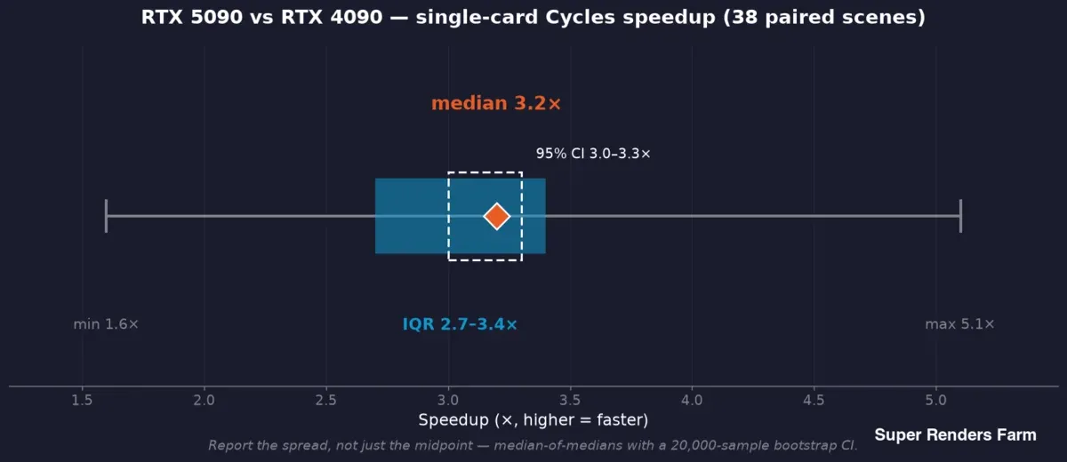
RTX 5090 versus RTX 4090 Einzelkarte Cycles-Beschleunigung über 38 abgestimmte Szenen: Median 3,2-fach, 95%-Konfidenzintervall 3,0 bis 3,3-fach, Interquartilsabstand 2,7 bis 3,4-fach, Gesamtspanne 1,6 bis 5,1-fach
Wir verwenden einen Median der Mediane: Jede Szene liefert den Median ihrer eigenen Pro-Frame-Zeiten auf jeder Seite, und die Schlagzeilen-Zahl ist der Median dieser Pro-Szene-Verhältnisse — sodass ein langsamer Frame das Ergebnis nicht verzerren kann. Um diesen Mittelpunkt herum berichten wir ein Bootstrap-Konfidenzintervall (die Feldstudie verwendete einen 20.000-Stichproben-Bootstrap, der ein 95%-KI von 3,0–3,3-fach um den Median von 3,2-fach ergab) sowie die Streuung — Interquartilsabstand 2,7–3,4-fach, Gesamtspanne 1,6–5,1-fach über diese 38 Szenen.
Diese Streuung ist kein Rauschen, das weggemittelt werden soll; sie ist das Ergebnis. Ein typischer 3,2-facher Geschwindigkeitsvorteil und ein 1,6-facher Worst-Case in einer Szene sind gleichzeitig wahr, und ein Benchmark, der nur den Mittelpunkt berichtet, versteckt die Hälfte der Geschichte, die ein Betreiber braucht. Die Regel, an der wir festhalten: Median und Spanne berichten und jede Behauptung an die Stichprobe knüpfen, die sie belegt — Beschleunigung aus 38 abgestimmten Szenen, VRAM aus 57 protokollierten Jobs, Leistungsaufnahme aus einem separaten kontrollierten Bench-Lauf, niemals eine Stichprobe zur Stützung einer anderen.
Wie man diesen Benchmark reproduziert
Das ist der Teil, der einen Benchmark zu einem verdienbaren Signal statt einer Marketingaussage macht: Jeder kann ihn durchführen. Die nachstehenden Schritte reproduzieren die Methode auf jeder Warteschlange oder jedem Testaufbau.
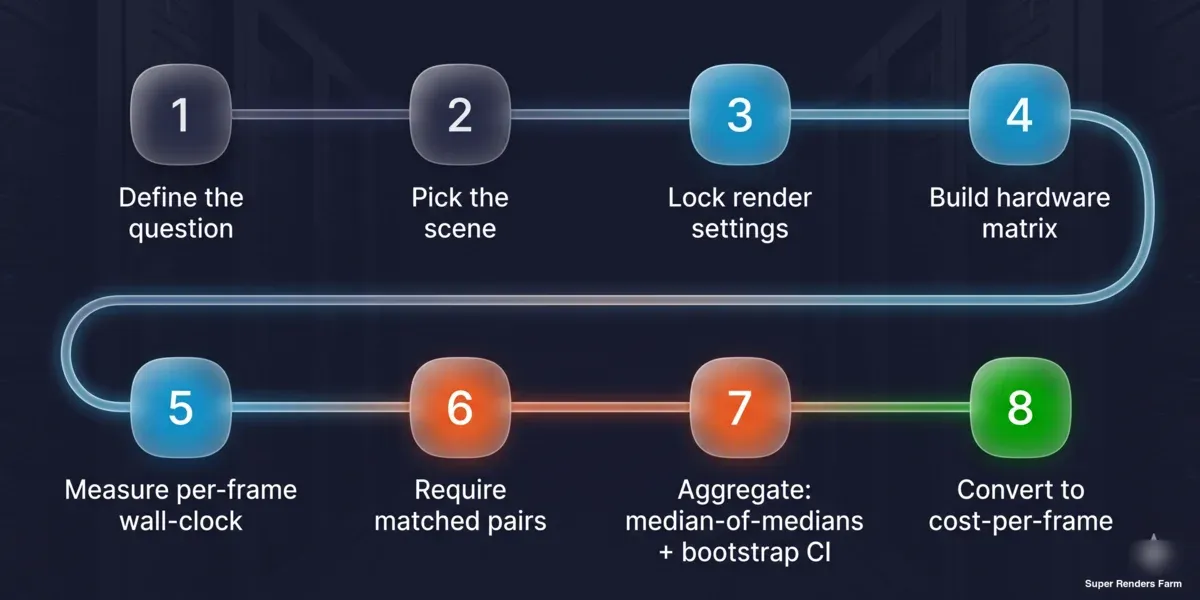
Achtschrittiger reproduzierbarer Kosten-pro-Frame-Benchmark: Frage definieren, Szene wählen, Render-Einstellungen sperren, Hardware-Matrix aufbauen, Wanduhrzeit pro Frame messen, abgestimmte Paare fordern, mit Median der Mediane und Bootstrap-Konfidenzintervall aggregieren, in Kosten pro Frame umrechnen
- Die Frage definieren. Maschinen-übergreifendes Ranking oder produktionsbasierte Kosten pro Frame? Die Antwort bestimmt den Szenentyp — Herstellerstandard für das Ranking, produktionsrepräsentativ für die Kosten.
- Szene und Einstellungen festlegen. Sampleanzahl oder Rausch-Schwellenwert, Denoiser-Auswahl, Ausgabeauflösung, Kachel-/Bucket-Größe und Engine-Build sperren. Aufschreiben; sie sind Teil des Ergebnisses.
- Die Matrix aufbauen. Karten auf einer Achse, Engine-/Szenen-Kombinationen auf der anderen auflisten. Festlegen, was konstant gehalten wird (Betriebssystem, Engine-Build, Denoiser, Szene), und aufzeichnen, was es nicht kann (Treiber).
- Wanduhrzeit pro Frame messen. Taskzeit ÷ Frameanzahl vom Scheduler oder einer Stoppuhr über den gesamten Job verwenden — nicht den internen Renderzeit-Wert der Engine, der Load- und Build-Overhead auslässt.
- Abgestimmte Paare und eine Mindest-Stichprobe fordern. Für jede A-versus-B-Behauptung dieselbe Szene auf beiden Seiten laufen lassen, mindestens drei Tasks pro Seite, bevor es zählt.
- Mit Median der Mediane aggregieren. Median jeder Szene pro Seite nehmen, dann den Median der Pro-Szene-Verhältnisse. Ein Bootstrap-Konfidenzintervall berechnen und Interquartilsabstand sowie Gesamtspanne daneben berichten.
- In Kosten pro Frame umrechnen. Gemessene Wanduhrzeit pro Frame mit Knotenkosten pro Stunde multiplizieren. Einheiten explizit halten, damit die Zahl prüfbar ist.
- Vorbehalte zusammen mit der Zahl veröffentlichen. Stichprobengröße hinter jeder Behauptung, Treiber-Situation, ob die Daten beobachtend oder kontrolliert sind, und den abgedeckten sowie nicht abgedeckten Geltungsbereich angeben.
Ein Studio, das diese acht Schritte auf seiner eigenen Hardware durchführt, erhält eine Zahl, die es verteidigen kann — und unsere damit überprüfen kann, was der Sinn der Veröffentlichung der Methode ist.
Hinweise zur Ehrlichkeit: Was ein Benchmark behaupten kann und was nicht
Eine Methode ist nur so vertrauenswürdig wie die Behauptungen, die sie ablehnt. Drei Linien, an denen wir festhalten:
Beobachtend ist nicht kontrolliert. Produktionsfelddaten — Jobs, die Nutzer im normalen Geschäftsbetrieb ausgeführt haben — sind real und nützlich, aber Nutzer passen ihre eigenen Szenen zwischen Re-Renders an, sodass es sich um beobachtende Daten handelt. Ein sauberer gleichzeitiger Vergleich (z. B. eine RTX 5090 gegen eine aktuelle RTX 4090 auf identischer Hardware) ist eine separate kontrollierte Übung. Wir lassen das eine nicht für das andere gelten.
Knoten-versus-Knoten enthält Setup, nicht nur Silizium. Wenn eine Seite auf Bare Metal und die andere virtualisiert läuft, ist ein Teil des gemessenen Abstands das Setup, nicht der Chip. Das gehört in den Schlagzeilen-Vorbehalt, nicht in eine Fußnote.
Keine Zahl, die wir nicht gemessen haben. Wir extrapolieren keine Leistungs- oder Thermik-Werte, die wir nicht gemessen haben. Wo unsere Feldstudie etwa 360–375 W pro Karte berichtet, stammt das aus einem kontrollierten Bench-Lauf unter anhaltender Last — und die daraus abgeleitete Energie-pro-Frame-Zahl ist als Schlussfolgerung, nicht als Messung gekennzeichnet. Wenn eine Zahl nicht gemessen wurde, erfindet die Methode sie nicht. Diese Disziplin ist der Grund, warum ein veröffentlichter Benchmark überhaupt zitiert werden kann.
Praxisbeispiele von unserer render farm
Diese Methode hat die nachstehenden Studien hervorgebracht; jede ist ein Datensatz, den Sie neben dem Rezept lesen können, und der richtige Ort für die tatsächlichen Zahlen, statt sie hier neu herzuleiten.
| Studie | Was die Methode ergab | Stichprobe |
|---|---|---|
| Multi-GPU-Skalierung | 1x→2x-Skalierung pro Engine auf Herstellerstandard-Szenen | 2 Knoten, 4 Engines, 7 Szenen-/Benchmark-Kombinationen |
| RTX-5090-Feldnotizen | Produktionskosten-/Beschleunigungsverteilung, VRAM-Perzentilen | 38 abgestimmte Szenen / 1.419 Tasks, 7 Wochen |
| V-Ray-Benchmark-Leitfaden | Schätzung Synthetischer Wert → Renderzeit | Referenztabellen und Rechenbeispiel |
| Cinebench für Cloud-Rendering | Interpretation synthetischer Werte für Hardware-Tiers | Referenzwerte |
Derselbe Ansatz liegt dem Kapazitätsplanen auf unserer GPU-Cloud-Render-Farm zugrunde, und die Blender-spezifischen Zahlen fließen in unsere Arbeit zum Blender-Cloud-Rendering ein — GPU ist ein Minderheitsanteil unseres Gesamt-Job-Mix (der Großteil der render-farm-Arbeit ist nach wie vor CPU-Rendering), deshalb begrenzen wir diese GPU-Zahlen genau darauf und machen daraus keine render-farm-weite Behauptung.
FAQ
Q: Wie benchmarkt man eine render-farm-GPU richtig? A: Entscheiden Sie zunächst, ob Sie ein maschinen-übergreifendes Ranking oder produktionsbasierte Kosten pro Frame anstreben. Für das Ranking verwenden Sie eine wiederholbare Herstellerstandard-Szene und einen festen Benchmark-Build. Für Kosten pro Frame verwenden Sie eine produktionsrepräsentative Szene, messen die Wanduhrzeit pro Frame (Taskzeit ÷ Frameanzahl) und multiplizieren mit den Knotenkosten pro Stunde. Sperren Sie die Render-Einstellungen und berichten Sie die Streuung, nicht nur eine einzelne Zahl.
Q: Warum sind Kosten pro Frame besser als ein Benchmark-Wert? A: Ein synthetischer Wert blendet alles aus, was sich in der Produktion verändert — Ihre Geometrie, Ihr Sampling, Ihren Denoiser und Ihre Auflösung —, sodass zwei Karten ähnlich abschneiden und dennoch bei Ihren Szenen stark unterschiedliche Kosten pro Frame aufweisen können. Kosten pro Frame ist die Einheit, in der ein Renderbudget tatsächlich aufgestellt wird, weshalb eine Methodik darauf hinauslaufen sollte statt auf einen Leaderboard-Punkt.
Q: Wie rechne ich einen Benchmark-Wert in eine Renderzeit-Schätzung um? A: Verwenden Sie das Verhältnis der Werte als groben Geschwindigkeitsquotienten: Eine Maschine, die auf demselben Benchmark-Build doppelt so viele Punkte wie eine andere erreicht, rendert einen vergleichbaren Frame in etwa der halben Zeit. Berechnen Sie die Effizienz Ihrer Maschine als Framezeit geteilt durch Benchmark-Wert und skalieren Sie dann mit dem Wert der Zielmaschine. Halten Sie den Benchmark-Build konstant, da Werte aus unterschiedlichen Builds nicht vergleichbar sind.
Q: Welche Kontrollen machen einen GPU-Benchmark vertrauenswürdig? A: Führen Sie pro Karte einen einzigen Rendertask für saubere Pro-Karte-Zahlen aus, fordern Sie abgestimmte Paare (dieselbe Szene auf beiden Seiten, eine Mindestanzahl von Tasks bevor ein Ergebnis zählt), halten Sie Treiber und Engine-Build innerhalb eines Messfensters konstant und halten Sie die Denoiser-Einstellung über den Vergleich hinweg identisch. Aggregieren Sie dann mit einem Median der Mediane und berichten Sie Konfidenzintervall und Spanne.
Q: Wie viele Testszenen brauche ich für ein zuverlässiges Ergebnis? A: Wenige hochwertige abgestimmte Paare schlagen viele lose kontrollierte. In unserer Produktionsstudie bestanden 38 Szenen einen strengen Einschlussfilter (dieselbe Szene und derselbe Nutzer auf beiden Hardware-Seiten, mindestens drei Tasks pro Seite) aus 1.419 Tasks. Die relevante Stichprobengröße ist das, was Ihren Filter besteht, nicht die rohe Task-Anzahl — und Sie sollten beide berichten.
Q: Kann ich Ihren render-farm-GPU-Benchmark selbst reproduzieren? A: Ja — das ist die Absicht. Szene und Einstellungen festlegen, Hardware-Matrix aufbauen und dabei Betriebssystem, Engine-Build und Denoiser konstant halten, Wanduhrzeit pro Frame messen, abgestimmte Paare fordern, mit Median der Mediane plus Bootstrap-Konfidenzintervall aggregieren, in Kosten pro Frame umrechnen und die Vorbehalte zusammen mit der Zahl veröffentlichen. Die acht Replikationsschritte oben legen die vollständige Abfolge dar.
Q: Warum berichten Sie eine Spanne statt einer einzigen Beschleunigungszahl? A: Weil die Spanne Teil des Ergebnisses ist. Dieselbe Hardware kann bei einer kurzen, overhead-gebundenen Szene einen 1,6-fachen Gewinn und bei einer schweren, rechengebundenen über das 5-fache zeigen, da feste Pro-Frame-Overhead-Kosten bei kurzen Renders einen größeren Anteil ausmachen. Nur den Mittelpunkt zu berichten verbirgt die Streuung, die ein Betreiber für die Kapazitätsplanung braucht — deshalb veröffentlichen wir Median, Interquartilsabstand und Gesamtspanne gemeinsam.
About Richard Ta
Richard Ta is co-founder and technical lead of Super Renders Farm (superrendersfarm.com), a fully managed cloud render farm that supports Maya, 3ds Max, Cinema 4D, Blender, and Houdini across the major render engines. He has spent over a decade building and running large-scale CPU and GPU render infrastructure for studios in more than 50 countries.